Deriving Non-Uniform Smoothness Indicators (\(k\)) for WENO

In my GSoC 2026 project for MethodOfLines.jl, my goal is to bring native non-uniform grid support to the WENO scheme.

The classic WENO scheme is highly effective at handling shocks and steep gradients in PDEs. However, its standard derivation assumes that the distance between grid points (\(\Delta x\)) is always constant. Due to this assumption, standard implementations rely on fixed, pre-calculated fractions (such as \(13/12\)) to compute their smoothness indicators.

When we move to a non-uniform grid where the spacing changes from node to node, these fixed fractions no longer work, and the scheme loses its theoretical accuracy. We cannot use static numbers; we need to dynamically recalculate the smoothness indicators (often denoted as \(\beta\) or \(k\)) for each specific grid interval.

In this technical blog post of my GSoC journey, I will focus directly on this problem. I will walk through how the actual derivation of non-uniform smoothness indicators is done from scratch using Lagrange interpolation.

1. The Geometry of a Non-Uniform Grid

Often, when deriving numerical schemes, a 1D computational domain is discretized into equal intervals. In such a uniform grid, the distance between any two adjacent points is a global constant, \(\Delta x\):

\[x_i - x_{i-1} = \Delta x \quad \text{for all } i\]

In a non-uniform domain, this comforting assumption vanishes. Points cluster tightly in areas with steep physical gradients (like boundary layers or shock waves) and spread out in smooth regions to save computational power. Therefore, \(\Delta x\) is no longer a single scalar number; every interval has its own unique identity and length.

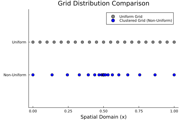
To build our mathematical foundation, let's isolate a local subset of this grid—a stencil. For a 5th-order WENO scheme, we operate on a 5-point global stencil (\(x_{i-2}\) to \(x_{i+2}\)), which is divided into three 3-point sub-stencils.

Let's define the exact coordinates of our nodes and the distinct, variable distances between them. Instead of a universal \(\Delta x\), we define the local step sizes as \(h\):

\[h_1 = x_{i-1} - x_{i-2}\] \[h_2 = x_i - x_{i-1}\] \[h_3 = x_{i+1} - x_i\] \[h_4 = x_{i+2} - x_{i+1}\]

When we derive the smoothness indicators for each sub-stencil, we can no longer factor out and cancel a common \(\Delta x\). Every geometric distance (\(h_1, h_2, h_3, h_4\)) must be explicitly carried through the entire integration process. This is the exact reason why the classic fractional weights break down, and it is where our derivation must begin.

2. What Exactly is "Smoothness"?

Before deriving the non-uniform formulas, we must define what we mean by "smoothness." In 1996, Jiang and Shu introduced a mathematical approach to measure how much a polynomial oscillates within a specific target cell.

To quantify this fluctuation, we look at the polynomial's derivatives. By squaring these derivatives, we ensure that positive and negative slopes do not cancel each other out, effectively measuring the total "energy" of the variations. Integrating these squared derivatives over the cell boundaries gives us the total accumulated fluctuation within that specific region.

For a polynomial \(P(x)\) of degree \(k\) (where \(k=2\) for a 5th-order WENO scheme), the smoothness indicator \(\beta\) over a target cell \(I_i = [x_{i-1/2}, x_{i+1/2}]\) is defined by the following integral:

\[ \beta = \sum_{l=1}^{k} h^{2l-1} \int_{x_{i-1/2}}^{x_{i+1/2}} \left( \frac{d^l}{dx^l} P(x) \right)^2 dx \]

In this formula, \(l\) represents the order of the derivative, and \(h\) is the length of the target cell (\(x_{i+1/2} - x_{i-1/2}\)). The scaling factor \(h^{2l-1}\) ensures that the smoothness indicator scales correctly with the grid size, keeping the values mathematically consistent regardless of how fine or coarse the grid is.

This integral is the core engine of our derivation. In the next step, we will construct our non-uniform polynomial \(P(x)\) using Lagrange interpolation and feed it directly into this engine.

3. Constructing the Polynomial via Lagrange Interpolation

To calculate the smoothness indicator, we first need the polynomial \(P(x)\) itself. For a 5th-order WENO scheme, the 5-point global stencil is split into three 3-point sub-stencils. Let's focus on the leftmost sub-stencil, denoted as \(S_0 = \{x_{i-2}, x_{i-1}, x_i\}\).

Our goal is to construct a 2nd-degree parabola, \(P_0(x)\), that passes exactly through the known function values at these three points: \(u_{i-2}\), \(u_{i-1}\), and \(u_i\). The most direct and robust mathematical tool for this is Lagrange Interpolation.

The standard form of a 2nd-degree Lagrange polynomial is:

\[ P_0(x) = u_{i-2} L_{i-2}(x) + u_{i-1} L_{i-1}(x) + u_{i} L_{i}(x) \]

Here, the basis polynomials (\(L\)) are determined entirely by the grid geometry. Let's write the first basis polynomial, \(L_{i-2}(x)\), explicitly:

\[ L_{i-2}(x) = \frac{(x - x_{i-1})(x - x_i)}{(x_{i-2} - x_{i-1})(x_{i-2} - x_i)} \]

Now, recall the local step sizes we defined in Step 1. We know that \(x_{i-1} - x_{i-2} = h_1\), which means the first term in the denominator is \(-h_1\). Similarly, the distance from \(x_{i-2}\) all the way to \(x_i\) is \(-(h_1 + h_2)\).

By applying these exact geometric distances to the denominators of all three basis polynomials, we obtain our fully non-uniform interpolation polynomial:

\[ P_0(x) = u_{i-2} \frac{(x - x_{i-1})(x - x_i)}{h_1(h_1 + h_2)} - u_{i-1} \frac{(x - x_{i-2})(x - x_i)}{h_1 h_2} + u_i \frac{(x - x_{i-2})(x - x_{i-1})}{h_2(h_1 + h_2)} \]

Notice how the denominators are now entirely composed of our variable step sizes. If this were a uniform grid, \(h_1\) and \(h_2\) would both simply be \(\Delta x\), and the denominators would trivially reduce to \(2\Delta x^2\), \(-\Delta x^2\), and \(2\Delta x^2\). In our non-uniform derivation, however, we strictly preserve the generic \(h\) terms to account for any arbitrary grid stretching.

4. Taking the Derivatives: Preparing for the Integral

To compute the smoothness indicator \(\beta_0\) using the Jiang-Shu formula from Step 2, we need the first (\(l=1\)) and second (\(l=2\)) derivatives of our interpolation polynomial \(P_0(x)\).

Let's start with the first derivative, \(P'_0(x)\). Taking the derivative of the numerator terms \((x - x_A)(x - x_B)\) using the product rule simply gives \((x - x_B) + (x - x_A)\), which simplifies to \(2x - x_A - x_B\).

Applying this to our polynomial, the first derivative becomes:

\[ P'_0(x) = u_{i-2} \frac{2x - (x_{i-1} + x_i)}{h_1(h_1 + h_2)} - u_{i-1} \frac{2x - (x_{i-2} + x_i)}{h_1 h_2} + u_i \frac{2x - (x_{i-2} + x_{i-1})}{h_2(h_1 + h_2)} \]

Notice that the first derivative is a linear function; it still depends on \(x\). This means when we square it and integrate it over the cell boundaries, we will be integrating a quadratic function.

Now, let's take the second derivative, \(P''_0(x)\). Differentiating \(2x - (\text{constants})\) simply leaves us with \(2\). The \(x\) variable completely disappears:

\[ P''_0(x) = u_{i-2} \frac{2}{h_1(h_1 + h_2)} - u_{i-1} \frac{2}{h_1 h_2} + u_i \frac{2}{h_2(h_1 + h_2)} \]

This is a beautiful mathematical simplification. The second derivative is completely independent of \(x\); it is a pure constant determined entirely by the grid geometry (\(h_1, h_2\)) and the nodal values (\(u\)). This means the second part of our Jiang-Shu integral (where \(l=2\)) will be remarkably easy to evaluate, as the integral of a constant squared over an interval is just the constant squared multiplied by the interval length.

With our derivatives ready, we can now feed them into the integral engine.

5. The Grand Integral Operation: Opening the Black Box

It is a common habit in papers to present the derivative polynomials and then immediately jump to the final \(\beta\) formulas "After performing the integration, we obtain..."

We will not do that. To truly understand how the non-uniform geometry affects the scheme, we must look inside this integration process.

To evaluate the integral without creating a mountain of unreadable algebra, we use a classic mathematical trick: a local coordinate shift. By setting our current node \(x_i\) as the origin (\(x_i = 0\)), the absolute coordinates disappear, and we are left strictly with our geometric distances (\(h\)):

• \(x_i = 0\)

• \(x_{i-1} = -h_2\)

• \(x_{i-2} = -(h_1 + h_2)\)

In a finite difference WENO scheme, the target cell \(I_i\) is typically centered around \(x_i\), with boundaries at the midpoints of the adjacent intervals. Therefore, our integration bounds become \([-h_2/2, h_3/2]\). The length of this target cell is \(\Delta x_i = \frac{h_2 + h_3}{2}\).

Let's explicitly evaluate the second-derivative part (\(l=2\)) of the Jiang-Shu formula from Step 2. Remember from Step 4 that \(P''_0(x)\) is a pure constant. Let's call this constant \(C\). The integral becomes incredibly straightforward:

\[ \text{Integral}_{l=2} = (\Delta x_i)^3 \int_{-h_2/2}^{h_3/2} (C)^2 dx \]

Since the integral of a constant over an interval is just the constant multiplied by the interval's length:

\[ \text{Integral}_{l=2} = (\Delta x_i)^3 \cdot C^2 \cdot \left( \frac{h_3}{2} - \left(-\frac{h_2}{2}\right) \right) = (\Delta x_i)^3 \cdot C^2 \cdot \Delta x_i = (\Delta x_i)^4 \cdot C^2 \]

Now, substituting our actual constant \(C\) (which is \(P''_0(x)\) from Step 4), the \(l=2\) component of our smoothness indicator is explicitly:

\[ (\Delta x_i)^4 \left( u_{i-2} \frac{2}{h_1(h_1 + h_2)} - u_{i-1} \frac{2}{h_1 h_2} + u_i \frac{2}{h_2(h_1 + h_2)} \right)^2 \]

The first-derivative part (\(l=1\)) follows the exact same logic. Since \(P'_0(x)\) is a linear function of the form \(Ax + B\), squaring it yields \(A^2x^2 + 2ABx + B^2\). Integrating this polynomial over \([-h_2/2, h_3/2]\) generates standard cubic and quadratic terms evaluated at the boundaries.

When we sum the \(l=1\) and \(l=2\) integrals, the final non-uniform smoothness indicator \(\beta_0\) emerges as a massive quadratic form. Instead of static fractions, it is structured as:

\[ \beta_0 = C_{00} u_{i-2}^2 + C_{11} u_{i-1}^2 + C_{22} u_{i}^2 + C_{01} u_{i-2}u_{i-1} + C_{02} u_{i-2}u_{i} + C_{12} u_{i-1}u_{i} \]

Here, every single coefficient (\(C_{mn}\)) is a dynamic function of our local grid spacings (\(h_1, h_2, h_3\)). The "black box" is gone: we now know exactly how the spatial geometry dictates the stability of the numerical scheme.

6. The Sanity Check: Return to the Magic Fractions

We have successfully derived a massive, fully dynamic formula for \(\beta_0\). But how do we know it is actually correct?

Let's perform a sanity check. What happens to our dynamic coefficients (\(C_{mn}\)) if we suddenly apply them to a perfectly uniform grid?

In a uniform grid, all step sizes are identical. Let's set \(h_1 = h_2 = h_3 = \Delta x\). If we substitute this assumption into the full algebraic expansion of our \(l=1\) and \(l=2\) integrals, something beautiful happens. All the complex algebraic terms gracefully cancel each other out, and the massive equation collapses into a very familiar form:

\[\beta_0 = \frac{13}{12} (u_{i-2} - 2u_{i-1} + u_i)^2 + \frac{1}{4} (u_{i-2} - 4u_{i-1} + 3u_i)^2\]

The "magic" fractions—\(13/12\) and \(1/4\)—suddenly reappear!

They were never universal constants of nature; they were just the specific geometric shadows cast by a uniform grid. By keeping our derivation purely in terms of local \(h\) distances, we have proven that our non-uniform engine is completely backward-compatible. It seamlessly becomes the classic WENO scheme when the grid is uniform, but dynamically adapts without failing when the grid stretches.

7. From Mathematics to Code: Implementation Strategies

Now that we have derived the generalized \(\beta_0\) for any non-uniform stencil, we face a critical software engineering problem: How do we effectively translate this massive mathematical equation into a performant PDE solver?

If we manually expand all the \(C_{mn}\) coefficients from Step 5, we end up with hundreds of algebraic terms. Hardcoding these expanded equations into the inner loops of MethodOfLines.jl would be highly prone to human error and nearly impossible to maintain.

Instead of forcing the solver to perform these heavy algebraic evaluations step-by-step during the simulation, our current strategy revolves around generating these weights dynamically. By exploring approaches like Symbolic Abstract Syntax Tree (AST) generation, our goal is to pre-calculate these complex integrals based on the specific grid geometry before the actual time-stepping begins.

The primary objective here is to shift the computational burden to the initial setup and discretization phase. While achieving absolute zero allocation in complex non-uniform setups is a highly ambitious target, pre-compiling these dynamic weights into streamlined Julia expressions should significantly minimize runtime overhead.

Architecturally, we are structuring this as an isolated weight calculator contained entirely within the WENO module. This modular design ensures that the core PDE pipeline remains untouched and stable. Finally, by leveraging Julia's multiple dispatch system, we can seamlessly route uniform grids (StepRangeLen) to the highly optimized, legacy "magic fractions," while directing non-uniform grids (AbstractVector) to our new dynamic engine.

This transition from static fractions to a flexible, dynamic algebraic architecture represents a necessary evolution to handle the variable-grid physics demanded by modern scientific simulations.

In the next technical post, I will dive into the second part of this implementation: Dynamic Weight Calculation with Fornberg. We will shift our focus from smoothness indicators to the core stencil weights, exploring how we can compute them on-the-fly. Stay tuned!