What Non-Uniform WENO Actually Buys Us
GSoC 2026 · MethodOfLines.jl · Final DevLog
August 2026 · Quantitative showcase
At a glance
Scenario A — A viscous shock layer on \([-1,1]\): clustered WENO at \(N=129\) beats uniform WENO at \(N=257\) by roughly two orders of magnitude.
Scenario B — A compressing interfacial front across two mismatched non-uniform subdomains: machine-precision seam continuity against an exact characteristic solution.
Takeaway — Under-resolving a steep feature on a uniform grid is a failure regime, not a convergence problem. Grid design is as important as the operator.
Introduction
My GSoC 2026 project for MethodOfLines.jl is complete. The goal was to bring native non-uniform grid support to the WENO-5 advection scheme. Earlier posts covered the smoothness indicators and the boundary architecture.
Many PDE problems contain localized steep gradients: shock-like transitions, boundary layers, or interfacial fronts. On a uniform grid, resolving one of these features means placing enough points everywhere to resolve it locally. Most of the grid then sits in regions where the solution is nearly flat. The cost scales with the global mesh, not with the feature.
There is a second issue. Under-resolving a steep gradient on a uniform grid is not a small-error regime. When the layer width falls below the grid scale, the semi-discretization can become unstable. The simulation does not converge slowly; it fails. Non-uniform WENO addresses both problems by concentrating resolution where the physics demands it, while keeping a high-order, non-oscillatory reconstruction on stretched meshes.
The two scenarios below quantify that difference against exact solutions.
Scenario A — The Stationary Viscous Shock
The first problem is the viscous Burgers equation on \([-1, 1]\) with viscosity \(\nu = 2 \times 10^{-3}\):
\[ \frac{\partial u}{\partial t} + u \frac{\partial u}{\partial x} = \nu \frac{\partial^2 u}{\partial x^2}, \qquad u(t, \mp 1) = \pm 1. \]Nonlinear advection steepens the profile; diffusion regularizes it. The equation admits the exact steady state
\[ u_\infty(x) = -\tanh\left(\frac{x}{2\nu}\right), \]an interior layer of width \(\mathcal{O}(\nu)\) centered at \(x = 0\). With \(\nu = 2 \times 10^{-3}\), the layer is roughly \(0.01\) wide. It is a standard finite-difference prototype for a steep interfacial gradient at a known, fixed location.
The test protocol is deliberate. We initialize from the exact steady profile and integrate to \(t = 1\). A capable scheme holds the layer in place with small error and no spurious oscillation. A poor scheme smears it, shifts it, or becomes numerically unstable.
We compare three configurations:
| Scheme | Grid | Points |
|---|---|---|
| First-order upwind | Uniform | \(N = 129\) |
| WENO-5 | Uniform | \(N = 257\) |
| WENO-5 | Clustered | \(N = 129\) |
The clustered grid is built from a resolution density peaked at the layer. Points are placed at uniform quantiles of that density, so cell widths vary smoothly across the domain. In MethodOfLines.jl, the full setup is a standard PDESystem discretized with WENOScheme() on a custom grid vector:
using ModelingToolkit, MethodOfLines, OrdinaryDiffEq, DomainSets
using OrdinaryDiffEqSSPRK: SSPRK33

@parameters t x
@variables u(..)
Dt = Differential(t)
Dx = Differential(x)

ν = 2.0e-3
u_steady(x) = -tanh(x / (2ν))

function grid_from_density(a, b, n, ρ; nsamples = 5001)
    xs = range(a, b, length = nsamples)
    cdf = cumsum(ρ.(xs))
    cdf = (cdf .- cdf[1]) ./ (cdf[end] - cdf[1])
    xg = map(range(0, 1, length = n)) do l
        k = searchsortedfirst(cdf, l)
        k <= 1 && return float(xs[1])
        θ = (l - cdf[k - 1]) / (cdf[k] - cdf[k - 1])
        return xs[k - 1] + θ * (xs[k] - xs[k - 1])
    end
    xg[1] = a
    xg[end] = b
    return xg
end

cluster_density(x) = 1 + 30 * exp(-x^2 / (2 * 0.02^2))
xg = grid_from_density(-1.0, 1.0, 129, cluster_density)

eq = Dt(u(t, x)) ~ -u(t, x) * Dx(u(t, x)) + ν * Dx(Dx(u(t, x)))
bcs = [u(0.0, x) ~ u_steady(x), u(t, -1.0) ~ 1.0, u(t, 1.0) ~ -1.0]
domains = [t ∈ Interval(0.0, 1.0), x ∈ Interval(-1.0, 1.0)]
@named pdesys = PDESystem(eq, bcs, domains, [t, x], [u(t, x)])

disc = MOLFiniteDifference([x => xg], t; advection_scheme = WENOScheme())
prob = discretize(pdesys, disc)
The grid vector xg is the only non-standard input. Everything else follows the usual MethodOfLines workflow.
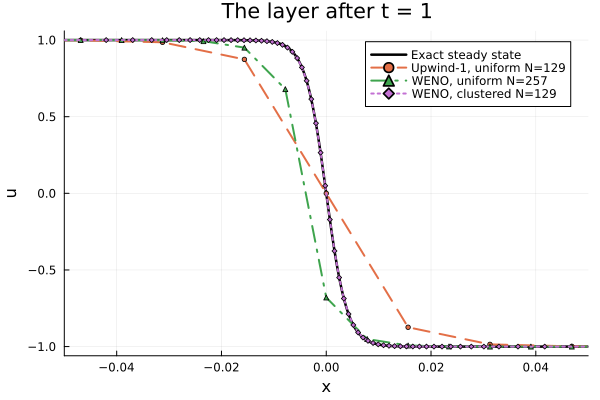
Figure 1. Profile zoom after \(t = 1\). Clustered WENO with \(N = 129\) tracks the exact steady state. Uniform WENO at \(N = 257\) remains non-oscillatory but visibly inaccurate. First-order upwind is dominated by numerical viscosity and resolves the wrong layer width.
Table 1. Relative \(L^2\) error after \(t = 1\).
| Configuration | Relative \(L^2\) error | Notes |
|---|---|---|
| Upwind-1, uniform \(N = 129\) | \(\approx 1.6 \times 10^{-2}\) | Numerical viscosity \(\gg\) physical \(\nu\); no convergence in this range |
| WENO, uniform \(N = 129\) | — | Unstable: sub-cell layer aborts the integration |
| WENO, uniform \(N = 257\) | \(\approx 4.6 \times 10^{-2}\) | Stable, but ~2 orders of magnitude worse than clustered |
| WENO, clustered \(N = 129\) | \(\approx 1.3 \times 10^{-4}\) | Overshoot at the \(10^{-8}\) level |
Key result. The clustered grid with half the degrees of freedom of the stable uniform WENO run delivers roughly two to three orders of magnitude lower error. The operator is the same; the grid design is not.
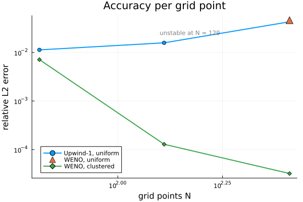
Figure 2. Relative \(L^2\) error versus grid points on a log-log scale. Clustered WENO converges cleanly across a self-similar refinement family. Uniform WENO appears as a single point at \(N = 257\) because the \(N = 129\) run is unstable. Upwind does not converge until \(N \gtrsim 1000\), when its numerical viscosity finally drops below the physical \(\nu\).
Scenario B — Interfacial Front Compression
The second problem moves from a single domain to a two-domain setup inspired by transport in a flow battery. Electrolyte enters from an open channel and flows into a porous electrode. Interstitial velocity decreases as porosity drops, and any concentration front carried by the flow compresses as it crosses the transition.
We model along-flow advection with a spatially varying slowness field
\[ s(x) = 1 + \left(\frac{1}{v_2} - 1\right) \frac{1 + \tanh((x - x_v)/\delta_v)}{2}, \]which ramps smoothly from \(1\) to \(1/v_2 = 2\) across a transition zone. The exact solution follows from characteristics:
\[ c(x, t) = S(t - \tau(x)), \qquad \tau(x) = \int_0^x s(\xi)\, d\xi, \]where \(S\) is a smooth inlet signal. A front of temporal width \(w_t\) has spatial width \(v(x)\, w_t\). It enters at width \(0.02\) and leaves the transition at width \(0.01\).
The domain is split at \(x = 1/2\) into two subdomains with independently generated non-uniform grids. Domain 2 uses roughly twice the point density, because the compressed front lives there. Continuity at the seam is enforced algebraically. The interface is computational: the underlying velocity field \(v(x) = 1/s(x)\) is continuous across the full domain.
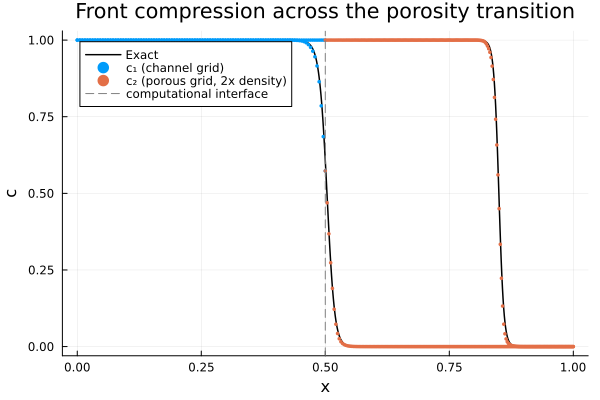
Figure 3. A steep front arrives at the seam at \(t \approx 0.67\), crosses onto a finer grid without a visible kink, and emerges at \(t = 1.3\) twice as steep. Numerical points track the exact characteristic solution on both sides.
Against the exact solution:
Seam continuity — Machine precision. The interface identification is algebraic, so \(|c_1 - c_2|\) at the seam is zero to floating-point tolerance.
Boundedness — The solution remains in \([0, 1]\) to within \(10^{-3}\) while the steep front crosses grids.
Accuracy — Weighted \(L^2\) error is below \(10^{-2}\) at both checkpoints. The mismatched non-uniform pair outperforms an evenly split uniform grid with the same total number of points.
This scenario exercises what multi-domain non-uniform grids are for: different subdomains carry different local feature scales, and the discretization must connect them without introducing artifacts at the seam. The velocity field must remain continuous across the interface; a genuine velocity jump destabilizes the cross-seam WENO stencil continuation. That is a limitation of the current non-conservative, node-centered formulation, not of the grid machinery itself.
Conclusion
The non-uniform WENO foundation in MethodOfLines.jl is now mathematically consistent and operationally complete: dynamic smoothness indicators on stretched stencils, boundary and interface handling, and end-to-end discretization on arbitrary rectilinear grids. The two scenarios above show where that matters. On a uniform grid, under-resolving a steep layer is a failure regime, not a convergence problem. On a clustered grid, the same operator resolves the feature accurately with far fewer global degrees of freedom. Across a multi-domain interface, independently designed non-uniform grids connect seamlessly while tracking a compressing front against an exact solution.
GSoC 2026 series
Showcase (this post)