Case study: laccase-catalysed oxidation of ABTS (measured data)
This page runs the one-call workflow on measured data: nine substrate-depletion progress curves of the oxidation of ABTS by a laccase, in triplicate, from an EnzymeML document published with the EnzymeML paper. It is the first real dataset the package has been run on. Nothing on this page runs in the test suite or in CI (it needs network access to download the data and about ten minutes of training); every number below comes from the run described in Results, in this environment.
Why this dataset and not the p53–Mdm2 loop
The case study planned for this release was the p53–Mdm2 negative-feedback loop, with the single-cell time series of nuclear p53 and Mdm2 fluorescence of Geva-Zatorsky et al. (2006), Molecular Systems Biology 2:2006.0033, or a later Lahav-laboratory dataset with both reporters. None was accessible from the environment in which this release was prepared: the journal site, PubMed Central, Zenodo, Dryad, Figshare, OSF, the laboratories' sites, and Cell Press were all unreachable (the network policy of the session allowed GitHub only), and no GitHub deposit of per-cell p53 and Mdm2 traces was found (the Lahav-laboratory repositories on GitHub hold tracking software without data, and the one repository with "p53 oscillations" in its name holds model simulations). The first fallback, the two ssrA-tagged fluorescent proteins competing for ClpXP of Cookson et al. (2011), Molecular Systems Biology 7:561, was unreachable for the same reason. The second fallback, a published enzyme progress-curve dataset with substrate depletion under saturating kinetics, was accessible on GitHub and is what this page uses. The p53–Mdm2 protocol is written out at the end of the page so that it can be run when the data are at hand.
Data
- Source:
Scenario4/ABTS_Measurement_Ngubane.omexin the GitHub repository EnzymeML/Lauterbach_2022, the supporting repository of Lauterbach, S. et al. (2023), "EnzymeML: seamless data flow and modeling of enzymatic data", Nature Methods 20, 400–402, doi:10.1038/s41592-022-01763-1. The document's creator is Sandile Ngubane (2021-10-15). - Format: an EnzymeML document (an OMEX archive: an SBML file with the species, reactions, and measurement metadata, and one CSV file per measurement).
- Content: laccase 2 (lap2, 0.93 µmol/l in every measurement, held constant) oxidising 2,2'-azino-bis(3-ethylbenzothiazoline-6-sulphonic acid) (ABTS). Nine measurements with nominal initial ABTS of 5, 10, 25, 35, 50, 65, 75, 110, and 150 µmol/l (the measured first points run from 6.3 to 154 µmol/l), each with 21 points at 60 s intervals from 0 to 1200 s and three replicates, observing the ABTS concentration in µmol/l. The document also declares an enzyme-inactivation reaction, which is not part of the model here.
- Download:
examples/laccase_abts/download_data.jlfetches the file from the repository at commit348b742f3c5f7e4e0d0a679b22ccd6b4d9bfdbe3(branchmain, 2022-04-11) and checks its SHA-256,d026cb2038c27e1bb7ceb7f4d60686b9a6feec6e92d1817aa9e6f9c09ff54975(10111 bytes), before unpacking it withunzip. - Licence: the repository has no licence file and the document no licence statement, so the data are not redistributed with the package; the download script and this page record where they come from. The article is open access under CC BY 4.0, which covers the article, not necessarily the repository. Cite the article above when using the data.
Preprocessing
examples/laccase_abts/preprocess.jl does the following and nothing else:
- Concentrations are divided by 100 µmol/l and times by 1000 s, so the model state is ABTS in units of 100 µmol/l and its time unit is 1000 s. Nothing is smoothed, trimmed, or interpolated; the 21 points of every replicate enter as measured. A global scale, rather than a per-curve normalisation, keeps the nine curves comparable, since they are absolute concentrations of the same substrate.
- Every replicate curve is one experiment (27 experiments); its initial condition is its own measured value at t = 0.
- The 25 µmol/l and 75 µmol/l curves (the third and seventh in order of initial concentration) are held out with all their replicates, six experiments of 27, about 22%. The rule was fixed before any run: two interior curves, so that the held-out residual measures interpolation between trained initial concentrations.
Model
One observed state, ABTS, with the per-concentration destruction rate unknown:
\[\frac{d[\mathrm{ABTS}]}{dt} = -D([\mathrm{ABTS}])\,[\mathrm{ABTS}],\]
declared as a reaction with known = false regulated by ABTS itself and, for clarity, as the edge ABTS → ABTS of kind UNKNOWN_NN. The enzyme concentration is the same in every curve, so it is not a state and is absorbed into D. The literature form for a single substrate and a constant enzyme is Michaelis–Menten depletion, -Vmax [ABTS] / (K + [ABTS]), which in this parametrisation is D = Vmax / (K + [ABTS]): a constant numerator over a denominator linear in ABTS, or a / (1 + b [ABTS]) with a = Vmax / K and b = 1 / K in the package's normalisation of the constant denominator coefficient. The compiled mechanism requires a production term, so a basal production of ABTS is declared with both of its parameters frozen during training at 1e-8 (the positivity constraint of the reference defaults does not admit zero), a production of 1e-16 model units per model time unit.
Recovered coefficients are in model units (ABTS per 100 µmol/l, rates per 1000 s). Because the enzyme concentration and the production scale are fixed rather than fitted, the scale of D is set by the data alone here; the identifiability diagnostic still runs and its numbers are reported.
Protocol
examples/laccase_abts/run_case_study.jl calls discover_unknown_terms twice with the reference defaults (warm-up on the first training experiment, Adam 100 then BFGS 50, the learned rate sampled on the regulator grid of the training experiments, bootstrap 8, discovery seed 3), once without and once with stability_selection = StabilitySelection() (100 resamples, τ = 0.8), with the six held-out experiments passed as holdout = 6 and the same random seed. Nothing is tuned per curve. examples/laccase_abts/plot_case_study.jl draws the figure from the files the run writes.
Results
Run on 2026-09-06 with Julia 1.10.12, OrdinaryDiffEq 7.8.1, SciMLSensitivity 7.119.2, Lux 1.31.4, Optimization 5.9.0, Zygote 0.7.13 (SciMLBase 3.50.2), 4 cores with four benchmark trainings running alongside: 208 s for the run with the reference defaults and 105 s for the run with stability selection (both train the same model; the second run's training finished faster because the first had compiled the code).
Training. The hybrid model fits the curves: final training loss 0.0020 (mean squared error in model units), root-mean-square error of the trained model against the data 3.8 µmol/l over the 21 training curves and 4.9 µmol/l over the 6 held-out curves (per curve, from 0.7 µmol/l at 5 µmol/l initial ABTS to 8.8 µmol/l at 150 µmol/l). The frozen production parameters stayed at 1e-8. The identifiability diagnostic reports a collinearity of 0.42 between the (frozen) production rate and the destruction scale and does not flag the edge; with no fitted production parameter the Fisher condition number is infinite, and the diagnostic is not informative here.
Discovery: no rational rate was accepted. With the reference defaults and with stability selection alike, the discovery returned DenominatorUnsafe: the sparse implicit fit selected a denominator that changes sign on the sample domain ("discovered denominator is singular on train/validation/domain data"), and the safety check rejected the candidate. There is no discovered equation, no hybrid residual, and no selection-frequency table (the stage runs after a candidate exists). The result is the same without the bootstrap, so it is not a bootstrap artefact.
Why. The learned per-concentration rate is not a decreasing function of ABTS, which Michaelis–Menten depletion with a constant enzyme would require. Sampled on the regulator grid (5 to 152 µmol/l, 80 points) it is non-monotone:
| ABTS (µmol/l) | 5 | 26 | 47 | 68 | 88 | 109 | 130 | 151 |
|---|---|---|---|---|---|---|---|---|
| learned D (1/s) | 0.00123 | 0.00189 | 0.00290 | 0.00188 | 0.00184 | 0.00250 | 0.00280 | 0.00290 |
The rate rises overall with concentration and has a bump near 47 µmol/l. The data themselves say why a one-state model cannot do better: every curve flattens at a non-zero concentration (about 2.5 µmol/l for the 5 µmol/l curve, 9 to 10 µmol/l for the 50 µmol/l curve, 26 to 28 µmol/l for the 150 µmol/l curve), and the fraction consumed in 1200 s is larger at high initial concentration (83% at 150 µmol/l, 60% at 6.5 µmol/l). A destruction rate that depends on the ABTS concentration alone, without time, cannot stop at a curve-dependent plateau: the trained model runs below the measured plateaus at late times (visible in the figure; the mean error of 3.8 µmol/l hides this systematic miss), its rate is a compromise across curves that produces the bumps, and no low-order rational function fits the bumps with a positive denominator. The source document's own model includes an enzyme-inactivation reaction, which is a time-dependent loss of activity that this one-state model does not represent.
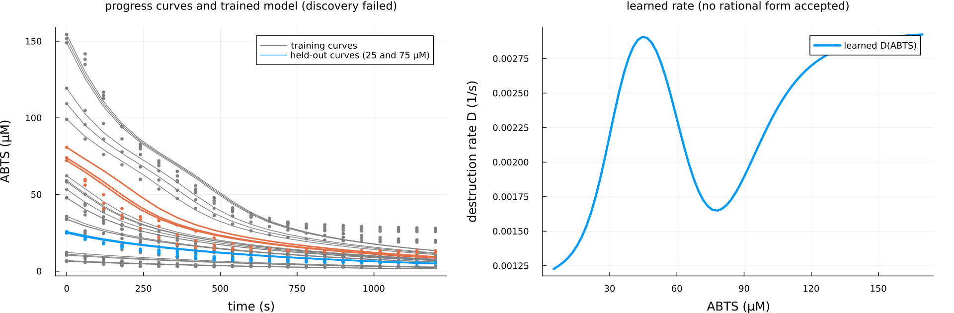
Comparison with the literature form. The discovered form cannot be compared, since none was accepted. The learned rate is the opposite of the literature form in its trend (increasing rather than decreasing in the substrate), which is the signature of a missing state rather than of a different kinetics.
What this does and does not show
This case study shows the workflow running end to end on measured data with the same defaults as the synthetic benchmarks: the data loader, the scaled units, the frozen production term, the held-out split, the training, and the discovery stage with its safety check. It shows the safety check doing its job: a rational rate that would have a pole on the data domain was refused rather than reported, and the failure is stated as such in the report. It does not show mechanism recovery on measured data, and it does not test the package's central claim (recovering a regulated destruction term from a partner state) because the accessible dataset has one observed state and no regulator. The two-state variants of the next section (0.13) take the next step, a latent enzyme state or a product dependence; the p53–Mdm2 study is on its own page. Nothing here was tuned: the run uses the reference defaults, and the only choices (units, held-out curves, the frozen production) were fixed before the first run and are listed above.
Two model variants (0.13)
The one-state result above is consistent with a missing state: enzyme inactivation, which the source document models, or product inhibition. Two variants were run on the same data, split, budget, and discovery configuration, one run each, nothing tuned per curve, no default changed (examples/laccase_abts/run_model_variants.jl, 2026-09-06, Julia 1.10.12, OrdinaryDiffEq 7.8.1, SciMLSensitivity 7.119.2, Lux 1.31.4, Optimization 5.9.0, Zygote 0.7.13, SciMLBase 3.50.2, 4 cores, with the p53 case study training alongside). Both have two regulators, so they run the same steps as the one-call workflow (warm-up on the first training curve, Adam 100 then BFGS 50, samples of the learned rate, the reference discovery configuration, hybrid residuals on the training and held-out curves) rather than the one-regulator entry point.
- (a) Product inhibition. States ABTS and C, the curve's initial concentration, a state with no reactions (dC/dt = 0), so that the product Q = C − ABTS is a function of the two; the unknown destruction of ABTS reads ABTS and C (the graph edges are derived from the reaction). The rate is sampled on a design over (ABTS, C): for each of the nine initial concentrations, 10 values of ABTS from that curve's last measured value to its first (90 points per replicate set, 210 points). Training: 261 s, final loss 0.00050; trained-model RMSE 1.9 µmol/l over the training curves and 2.7 µmol/l over the held-out curves (the one-state model: 3.8 and 4.9). Discovery accepted a rational rate,
D = (1.54 + 2.56 S) / (1 + 0.503 S²)(S = ABTS per 100 µmol/l, rate per 1000 s), whose numerator and denominator use ABTS only: no term in C survived thresholding, so the accepted form does not use the product. Its hybrid-model RMSE is 3.3 µmol/l over the training curves and 2.7 µmol/l over the held-out curves. The form rises with ABTS at low concentration and falls at high concentration, which is not Michaelis–Menten depletion either; it is a description of the learned rate that the safety check accepts, with no product dependence. - (b) Enzyme inactivation. States ABTS and E, the active enzyme (unobserved, µmol/l, E(0) = 0.93 as in the source document), with first-order inactivation
k_inactfitted; the unknown destruction of ABTS reads ABTS and E. The rate is sampled along the trained model's trajectories of the training curves (every second point, 231 points). Training: 202 s, final loss 0.00071; fittedk_inact= 1.51 per 1000 s (an activity half-life of about 460 s); trained-model RMSE 2.5 µmol/l over the training curves and 4.1 µmol/l over the held-out curves. Discovery returnedDenominatorUnsafeagain: the selected denominator changes sign on the sample domain, and the safety check refused the candidate. No accepted rate.
What this adds: both variants fit the curves better than the one-state model, the product-inhibition variant the most, and one of them yields an accepted rational rate, but that rate uses the substrate alone and is not the literature form. The enzyme-inactivation variant fits a plausible inactivation rate and still gives no accepted rational rate in two variables. A dataset with the enzyme activity or the product measured would be needed to separate the two mechanisms; with ABTS alone, the data do not decide.
The p53–Mdm2 protocol
Run in 0.13 on measured p53 traces with Mdm2 unobserved; see Case study: the p53–Mdm2 loop. The protocol as planned: two states, p53 (P) and Mdm2 (M). Known: production of M activated by P as a mass-action term (the simplest form consistent with the delayed transcriptional activation of the 2006 model; a Hill form is the alternative), linear degradation of M, constant production of P. Unknown: the destruction term of P, regulated by M, declared as a reaction with known = false and the edge P ← M. Fluorescence units are arbitrary, so each trace would be normalised to its own maximum, and recovered coefficients would be in those units with the production/destruction scale not separately identifiable. Cells with sustained oscillations would be selected by the paper's criterion where stated and otherwise by a documented rule (for example at least four peaks in 48 h), resampled to a common grid, one experiment per cell, about 20% of cells held out, and discover_unknown_terms run with the reference defaults and then with stability selection, reporting the identifiability diagnostic, the training and held-out residuals, the learned destruction rate against M with the discovered rational form, and the selection frequencies; the discovered form would be compared with the Mdm2-mediated degradation term of the literature model (monotone in M, saturating or not).